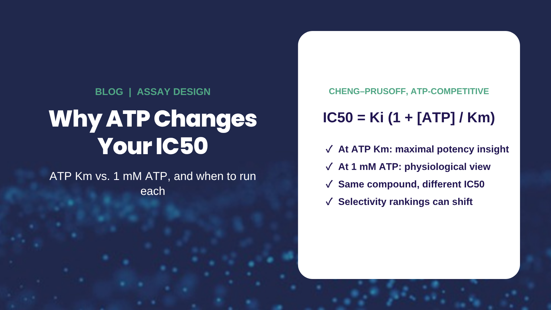
Two labs test the same ATP-competitive kinase inhibitor against the same kinase and report IC50 values that differ by 50-fold. Neither lab made a mistake. They ran their assays at different ATP concentrations.
ATP concentration is one of the most consequential and least discussed variables in kinase biochemistry. It changes measured potency, it can change the rank order of your off-targets, and it determines how well a biochemical result predicts what happens in cells. This post explains why, with a worked example, and lays out when to profile at ATP Km, when to profile at 1 mM ATP, and what to ask a profiling partner.
Key takeaways
- For an ATP-competitive inhibitor, measured IC50 rises as ATP concentration rises. The size of the shift depends on each kinase's Km for ATP.
- Profiling at ATP Km puts every kinase on equal footing (IC50 ≈ 2 × Ki), which makes it the right condition for comparing intrinsic affinity across the kinome.
- Profiling at 1 mM ATP approximates the millimolar ATP inside cells, so it is the better predictor of which off-targets survive in a cellular setting.
- Selectivity can look very different at low ATP versus 1 mM because kinases with low ATP Km values lose apparent potency faster.
- Inhibitors that are not ATP-competitive show little ATP-dependent shift, so comparing both conditions is also a quick mechanism check.
The relationship behind the shift
For an inhibitor that competes with ATP for the active site, the measured IC50 depends on the inhibitor's true affinity (Ki), the ATP concentration in the assay, and the kinase's Michaelis constant for ATP (Km,ATP). The Cheng–Prusoff relationship describes it:
IC50 = Ki × (1 + [ATP] / Km,ATP)
Two consequences follow. First, when [ATP] equals Km,ATP, IC50 equals 2 × Ki for every kinase, regardless of how tightly that kinase binds ATP. Second, when [ATP] is far above Km,ATP, IC50 grows roughly in proportion to ATP. Because Km,ATP varies widely across the kinome, from low micromolar to hundreds of micromolar, the same ATP concentration affects different kinases very differently.
A worked example: same inhibitor, two kinases, three ATP conditions
Consider an inhibitor that binds two kinases with identical affinity (Ki = 5 nM). Kinase A has a low ATP Km (10 µM). Kinase B has a high ATP Km (200 µM). Here is the IC50 you would measure under three common assay conditions:
| Assay condition | Kinase A (Km,ATP 10 µM) | Kinase B (Km,ATP 200 µM) | What it suggests |
|---|
| Fixed 10 µM ATP | 10 nM | 5.3 nM | Roughly equipotent |
| ATP Km for each kinase | 10 nM | 10 nM | Identical intrinsic affinity |
| 1 mM ATP | 505 nM | 30 nM | About 17-fold selective for B |
Nothing about the compound changed. At Km, the two kinases look identical, which is accurate: the inhibitor binds both equally well. At 1 mM ATP, kinase A's low Km means it is far more saturated with ATP, so the inhibitor struggles to compete and kinase A drops out as an off-target. That 1 mM picture is closer to what the compound will face inside a cell.
When to profile at ATP Km
ATP Km is the best condition for comparing intrinsic affinity across many kinases. Because IC50 ≈ 2 × Ki for every target, differences in your data reflect differences in binding rather than differences in each kinase's appetite for ATP. Use it for:
- Broad early selectivity screens where you want an unbiased view of every kinase your compound can engage
- Structure–activity relationship (SAR) work, where you need potency values that track binding changes across a series
- Comparing your data with literature or internal values reported as Ki
When to profile at 1 mM ATP
ATP inside cells is typically in the low millimolar range, far above the Km of most kinases. Profiling at 1 mM ATP approximates that competitive pressure, so it tells you which off-targets are likely to matter in cells. Use it for:
- Late-stage lead optimization and candidate selection, when you need to know which liabilities will survive physiological ATP
- Safety and off-target triage before cell-based or in vivo studies
- Explaining why biochemical potency and cellular potency disagree
Running both conditions on the same compound gives you the most complete picture: intrinsic affinity from Km data and likely cellular relevance from 1 mM data.
When ATP concentration matters less
The Cheng–Prusoff shift applies to ATP-competitive inhibitors. Inhibitors that bind outside the ATP site, such as allosteric (type III and IV) compounds, show little change in IC50 as ATP rises. If a compound's potency barely moves between Km and 1 mM ATP, that is a useful early hint that it may not compete with ATP, and it is worth confirming with mechanism-of-action studies.
Covalent and slow-binding inhibitors add another dimension: their IC50 also depends on how long the reaction runs. For these compounds, single-timepoint IC50 values can be misleading at any ATP concentration, and parameters such as kinact/KI from a time-dependent inhibition study describe potency more reliably. Our post on continuous vs. endpoint kinase assays explains why kinetic readouts catch these effects.
A caveat on biochemical vs. cellular selectivity
Even 1 mM ATP does not recreate a cell. Kinase conformation, scaffolding partners, and compound permeability all influence what an inhibitor does in situ. A 2026 study in the Journal of Medicinal Chemistry compared cell-free profiling with in-cell target engagement for ten kinase inhibitors and found results that diverged enough to change probe prioritization. Physiological ATP narrows the gap between biochemistry and cells, but it does not close it, which is why well-characterized biochemical data and cellular follow-up work best together.
Questions to ask your profiling partner
- What ATP concentration do you run by default, and is it the same for every kinase?
- Do you offer profiling at each kinase's ATP Km? At 1 mM? At a custom concentration?
- How were the Km values determined, and under what substrate and buffer conditions?
- Is the readout continuous or a single endpoint, and will I see progress curves?
- How do you flag time-dependent or non-ATP-competitive behavior in the report?
How AssayQuant handles ATP in KinSight™ profiling
Every target in our KinSight kinase and phosphatase panels is available at ATP Km, 1 mM ATP, or a custom concentration, and all panels run in duplicate. Because PhosphoSens® assays read out continuously, every well produces a full progress curve, so you can see time-dependent behavior instead of inferring it from one number. If you are deciding which condition fits your program, or want both, explore KinSight kinome profiling or talk to an AssayQuant scientist →
References
- Cheng Y, Prusoff WH. Relationship between the inhibition constant (K1) and the concentration of inhibitor which causes 50 per cent inhibition (I50) of an enzymatic reaction. Biochem Pharmacol. 1973;22(23):3099–3108. doi:10.1016/0006-2952(73)90196-2
- Knight ZA, Shokat KM. Features of selective kinase inhibitors. Chem Biol. 2005;12(6):621–637. doi:10.1016/j.chembiol.2005.04.011
- Binder MJ, et al. Cellular context influences kinase inhibitor selectivity. J Med Chem. 2026;69(4):4208–4220. doi:10.1021/acs.jmedchem.5c02916